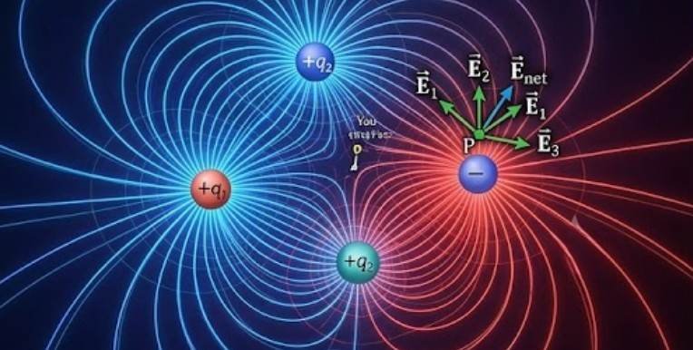
Two nearby charges can create a point where the net electric field is zero even though neither charge produces zero field there. That is the key idea behind electric field due to multiple point charges: individual fields overlap, and the final result depends on magnitude and direction.
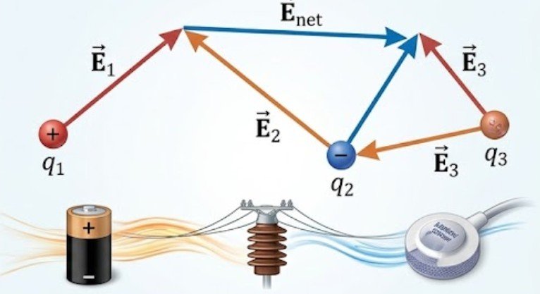
The governing rule is superposition. Each source charge creates its own electric field independently, and the net field at an observation point is the vector sum of those contributions. OpenStax explains this principle directly in its university-level treatment of electric fields.
The Principle That Makes Many-Charge Problems Manageable
For one point charge, the field magnitude at distance r is:
E = k|q|/r²
where k ≈ 8.99 × 10⁹ N·m²/C², q is the source charge, and r is the distance to the observation point. Some physics materials use the same Coulomb-law relationship and constant.
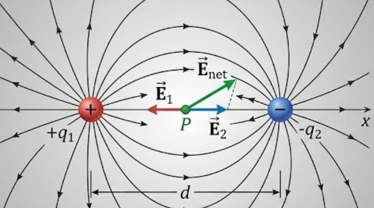
Direction matters just as much as magnitude. A positive charge creates a field pointing away from itself. A negative charge creates a field pointing toward itself.
For several charges:
E⃗_net = E⃗₁ + E⃗₂ + E⃗₃ + …
This is a vector equation. Adding 200 N/C and 150 N/C does not automatically give 350 N/C. If the vectors oppose one another, the result can be much smaller. Oregon State University similarly describes a many-charge electric field as the sum of the individual vector components.
A compact form is:
E⃗(P) = Σ [kqᵢ r⃗ᵢ / |r⃗ᵢ|³]
Here, r⃗ᵢ points from charge i to the observation point P.
A Six-Step Method That Works Consistently
1. Draw a Coordinate System
Put every source charge and the observation point on x-y axes. Record coordinates before calculating. This prevents sign errors later.
2. Find Each Displacement and Distance
If qᵢ is at (xᵢ, yᵢ) and the field is required at P = (x, y):
Δxᵢ = x – xᵢ
Δyᵢ = y – yᵢ
rᵢ = √[(Δxᵢ)² + (Δyᵢ)²]
Use meters in SI calculations.
3. Calculate Each Field Magnitude
For every charge:
Eᵢ = k|qᵢ|/rᵢ²
Do not add these magnitudes yet.
4. Assign the Direction
Imagine a tiny positive test charge at P. The field points in the direction that positive test charge would accelerate: away from +q and toward -q.
5. Resolve Each Field Into Components
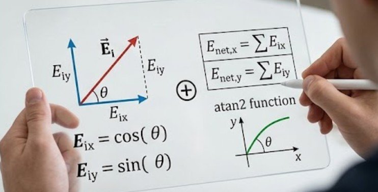
For a field at angle θ:
Eₓ = E cos θ
Eᵧ = E sin θ
A safer coordinate form is:
Eₓ,i = kqᵢΔxᵢ/rᵢ³
Eᵧ,i = kqᵢΔyᵢ/rᵢ³
Because qᵢ keeps its sign, this form automatically handles positive and negative charges.
6. Add Components and Reconstruct the Net Field
E_net,x = ΣEₓ,i
E_net,y = ΣEᵧ,i
Then:
|E_net| = √[(E_net,x)² + (E_net,y)²]
θ = atan2(E_net,y, E_net,x)
Using atan2 is safer than ordinary inverse tangent because it identifies the correct quadrant. HyperPhysics also cautions that basic arctangent calculations can produce quadrant ambiguity in multiple-charge problems.
Worked Example: Two Charges and an Off-Axis Point
Suppose:
q₁ = +3.0 nC at (-0.20 m, 0)
q₂ = -2.0 nC at (+0.20 m, 0)
Find the field at P = (0, 0.30 m).
Both charges are the same distance from P:
r = √[(0.20)² + (0.30)²] = 0.3606 m
For q₁:
E₁ = 8.99 × 10⁹(3.0 × 10⁻⁹)/(0.3606)²
E₁ ≈ 207 N/C
Because q₁ is positive:
E₁,x ≈ +115 N/C
E₁,y ≈ +173 N/C
For q₂:
E₂ ≈ 138 N/C
Because q₂ is negative, its field points toward q₂:
E₂,x ≈ +76.7 N/C
E₂,y ≈ -115 N/C
Add by direction:
E_net,x = 115 + 76.7 = 191.7 N/C
E_net,y = 173 – 115 = 57.5 N/C
Therefore:
|E_net| ≈ 200 N/C
θ ≈ 16.7° above the +x-axis.
The geometry explains the answer before the arithmetic is finished: the horizontal components reinforce each other, while the vertical components partially cancel.
Use Symmetry Before Reaching for a Calculator
Symmetry can shorten many electric field due to multiple point charges problems. If equal charges are placed symmetrically around a point, some components may cancel exactly.
For two identical positive charges the same distance left and right of a point on their perpendicular bisector, horizontal components cancel while vertical components add. OpenStax demonstrates this same component-cancellation principle in symmetric charge arrangements.
Interactive field maps can also help you check whether your predicted direction is physically sensible before trusting a long calculation. The University of Colorado Boulder provides a PhET simulation for exploring electric charges and fields visually.
Where the Point-Charge Method Has Limits
The model works best when charges can reasonably be treated as concentrated at individual locations. Charged rods, disks, surfaces, or volumes usually require integration rather than a finite sum.
The same superposition principle still applies, but the discrete sum becomes an integral over a line, surface, or volume. OpenStax’s treatment of continuous charge distributions shows how line, surface, and volume charge densities are handled mathematically.
Gauss’s law can sometimes simplify these calculations further when the geometry has sufficient symmetry.
Also remember that electric field is not electric force. Once the field is known, the force on a separate test charge Q is:
F⃗ = Q E⃗_net
A negative test charge experiences force opposite the electric-field direction.
Why the Method Matters
Superposition is the basis for predicting how charged particles behave in complex electrostatic environments. More practically, it turns a many-charge problem into repeated applications of one rule: calculate each contribution independently, preserve its direction, and then add the vectors.
The method also scales. Three, four, or ten point charges do not require a new law. They simply require more individual vector contributions.
Frequently Asked Questions
1. Can the electric field be zero between multiple charges?
Yes. Individual fields can cancel at locations where their vector contributions have equal magnitude and opposite direction.
2. Do electric fields from different charges interfere?
They superpose. Each charge contributes its own field, and the net field is the vector sum of all contributions at that point.
3. Why are components needed for electric field due to multiple point charges?
Because electric field is a vector. Components let you add fields pointing in different directions without losing sign or geometric information.
4. Is electric potential calculated the same way?
Not exactly. Electric potential is a scalar, so potentials add algebraically. Electric fields require vector addition.
Final Takeaway
More charges do not automatically mean a larger electric field. Direction can reinforce, weaken, or completely cancel individual contributions.
The most reliable habit is to draw the geometry, calculate one charge at a time, resolve every field into components, and add only after the directions are clear. If the final vector disagrees with the physical picture, recheck signs and geometry before redoing the arithmetic. Once superposition becomes a vector routine rather than a memorized formula, these problems become far more predictable.
Leave a Reply